Creating Fibonacci Patterns with Geometry Nodes

2024-09-26 · By Richard

Today we're going to use the Fibonacci sequence and the Golden Ratio to create a pattern that's similar to the seed arrangements found in flowers.

It's based on some very simple principles, but can create some interesting and complex looking patterns:

Below I'm walking through the steps to create this in Blender.

This is the first screencast, where I start from a fresh Blender scene and create a foundation of the flat pattern:

Here is the final .blend file I ended up with after this video: blendergrid-fibonacci-pattern-1-flat.blend

If you'd like to follow along in written form, you can check out the steps below.

When the pattern is done, we want to wrap it around a sphere. At that stage, I have another screencast because it involves quite a bit more trigonometry.

1. Introduction to the Fibonacci Sequence and Golden Ratio

The Fibonacci sequence is a series of numbers with a simple rule: Each number is the sum of the two preceding ones:

1, 1, 2, 3, 5, 8, 13, 21, 34, 55, 89, 144, ...

The Golden Ratio is related to this sequence. It can be approximated as the ratio of consecutive numbers. For example: 144 / 89 ~= 1.618

As the sequence continues, the ratio of consecutive numbers approximates the Golden Ratio (φ). This ratio is interesting because it appears frequently in nature, art, and architecture.

In this tutorial, we'll use the Golde Ratio to create patterns that look like seed arrangements found in flowers like sunflowers.

2. Initial Geometry Nodes Setup - Animating Points

Points are one of the most basic entities we can work with in Geometry Nodes. They only have a position and a radius. So for this pattern, I'd like to set it up with Geometry Nodes points.

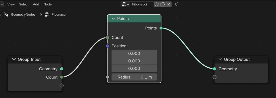
We'll use a Points node and make sure we can control the Point Count from the modifier interface:

Initially, we'll be setting up the Geometry Nodes to generate points that move out in a straight line along the X-axis.

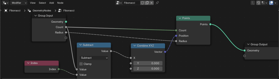
We pretty much use the Count of points to both set the Point Count and the X position of the first point. Then we make the next points follow the first point by subtracting their Index from their X position:

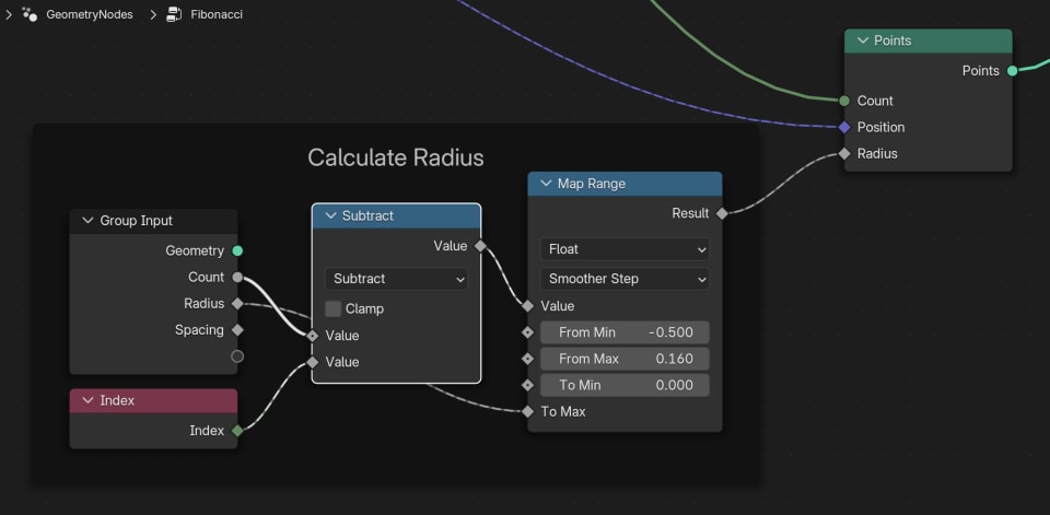
To make the points appaear a bit less abrupt, we'll make the radius of the points increase in the beginning. Making them grow from zero to their final size:

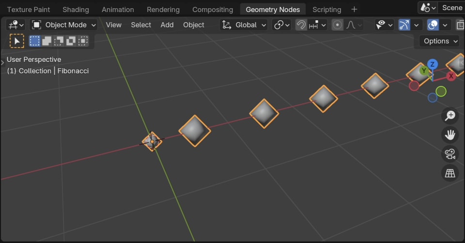
Now we have points moving out in a straight line along the X-axis as we increase the Count parameter:

3. Converting Linear to Circular

Now we turn this straight line of points into a spiral pattern.

Calculating the Polar Coordinates

Polar coordinates consist of an angle and a radius/distance. When placing the points in a straight line, we already have the distance component calculated. So all we need now is calculate an angle.

We can keep this super simple: Just choose one angle, say 20 degrees, and multiple each point's Index by this angle.

It's like we start moving the first point in a straight line, then move the next point in a line rotated 20° from the first line, the 3rd point is rotated 20° from the last line, etc.

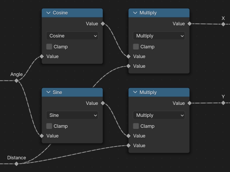
Once we have the distance and angle, we can use these to calculate the X and Y (Cartesian) coordinates using Sine and Cosine nodes:

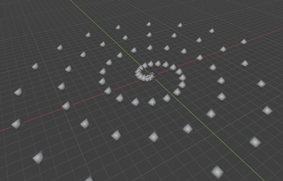
The result is a spiral pattern:

4. The Golden Angle

We can now choose any angle that we want to create different spiral patterns. It's cool to play with it and see what happens:

But if we want to mimic the way seeds are packed in a sunflower, we need the Golden Ratio to calculate a special Golden Angle.

The Golden Angle is pretty much 360° / φ where φ is the Golden Ratio. This is what we need to make the spiral pattern evenly distributed and looking natural.

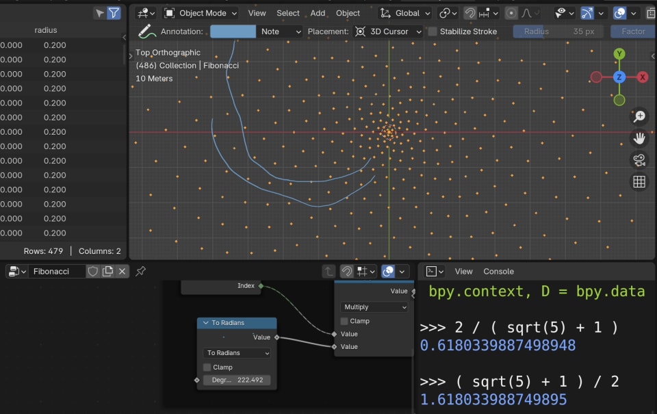
A formula for the Golden Ratio is:

φ = 2 / (√5 - 1)

So the Golden Angle in degrees is:

φ = 360 / φ = 180 * (√5 - 1)

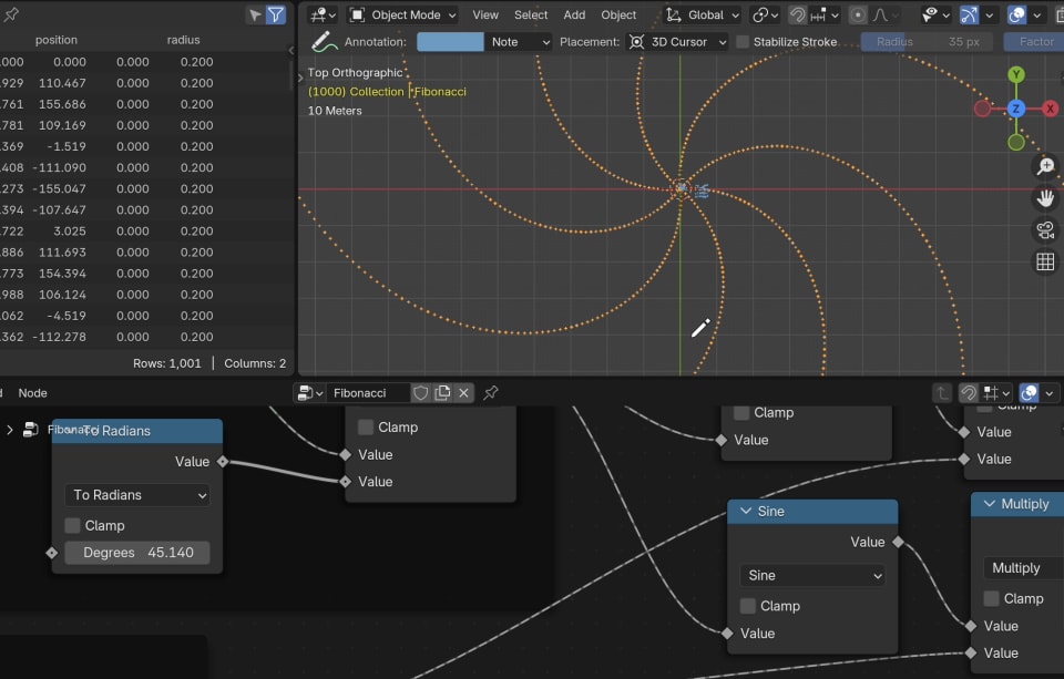
We could also calculate the Golden Angle in radians, but then we have to insert rounded values into the nodes, which reduces accuracy. Now, we only use whole numbers and we can let the nodes use all the precision they have to calculate our Golden Angle.

By rotating each point by the Golden Angle, we achieve a spiral pattern where points are evenly distributed, mimicking natural patterns:

5. Adjusting distance for better spacing

Now, the angle is great. But the points on the outside of the spiral are placed very far apart, while the points on the inside are close together.

This is simply because at every distance from the center, the amount of points at the circle with that distance is the same. But the circles are growing as they move outward.

So instead of constantly increasing the distance, we should try to constanctly increase the total area that each points covers. If that stays constant, the points will be evenly spaced.

The area is proportional to the square of the distance:

area ~ distance ^ 2

So if we want to know which distance we need to use, for a certain area, we can invert the formula:

distance ~ sqrt(area)

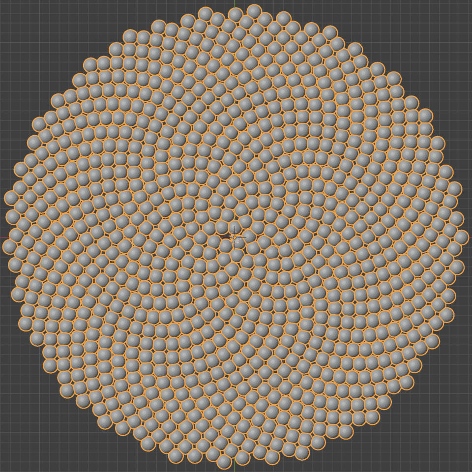
This is done by simply throwing a square root math Node into the mix:

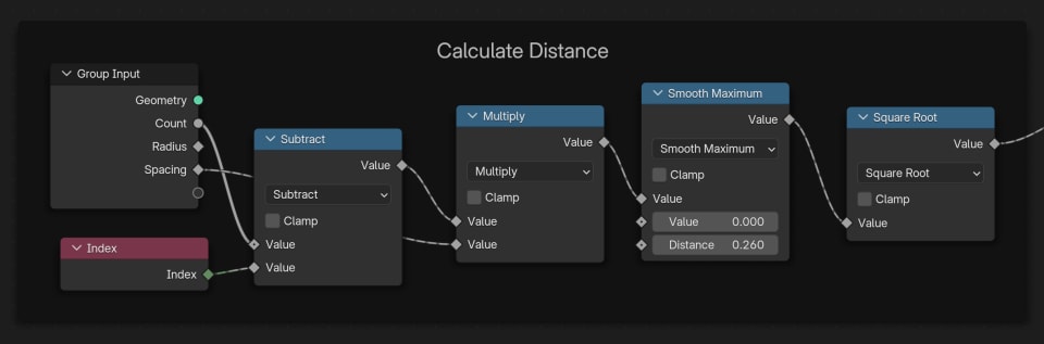
Now the pattern really starts to look like sunflower seeds:

6. Adding geometry on top of the points

Instead of points, let's use some actual geometry to make things look more interesting.

We can simply use an Icosphere node and an Instance on Points node to place Icospheres on top of the points.

Now we break the radius control, because the Instances on Points are not using the point radii. Instead of plugging our dynamic radius into the point raidus, we plug it into the scale of the Instances on Points node.

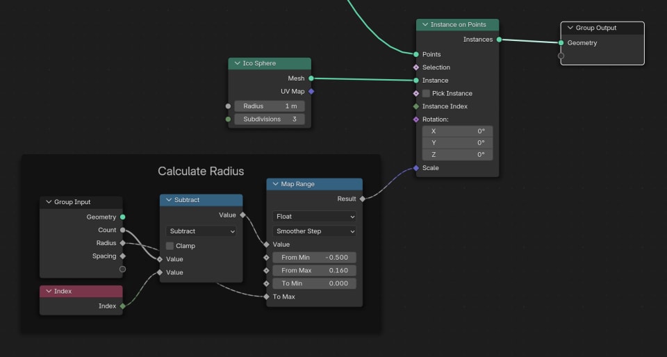
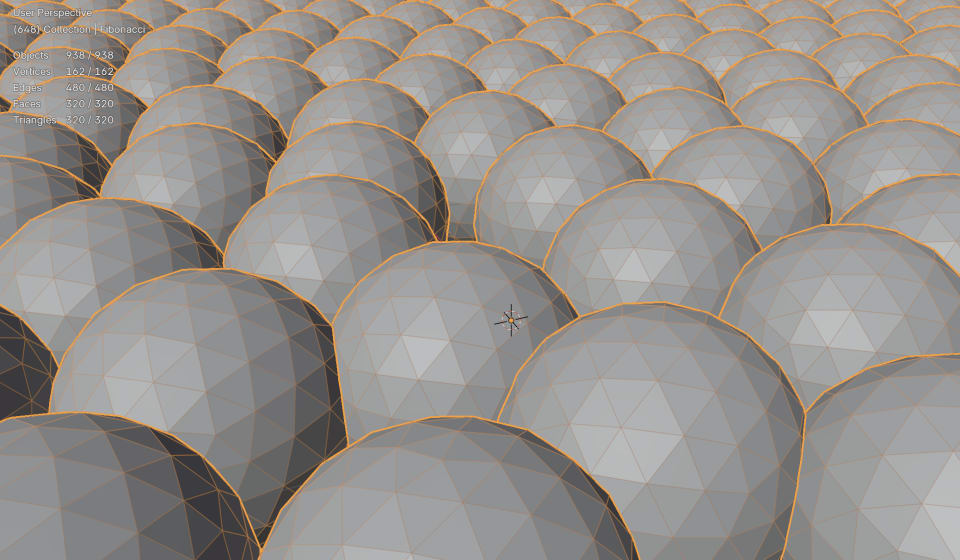
This gives us some actual meshes to render:

7. 4D Noise

Since we're working with a natural looking pattern, I'd like to add some randomness to make it look more organic.

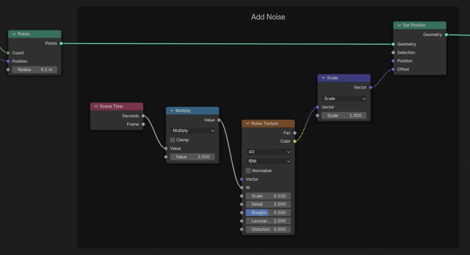
We can simply add a Set Position to the points and offset it with some Noise.

3D noise is based on the Positions of the points, so if we scale down the Noise, points that are positioned close together will be offset in a similar direction.

Instead of 3D noise, which makes the points offset in a random direction, we can use 4D noise, which makes the points offset in a random direction but we can make this direction slowly change over time. This is done by using the Scene Time node and plugging the value of seconds into the W component of the Noise Texture:

8. Animation

Let's make this pattern move.

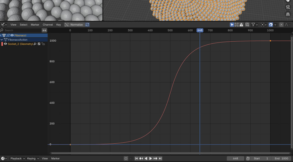
We can simply make the Count grow from 0 to 1000 using keyframes.

To make the animation look more interesting, You can use different interpolation methods for your keyframes. I'm using exponential interpolation and set the easing to Ease In and the easing to Ease In and Out. This way the movement starts off super slow, speeds up, and slows down again at the end.

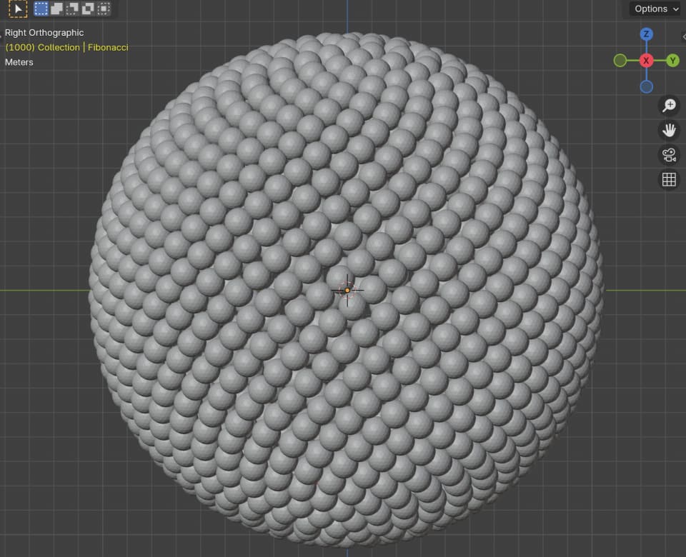
9. Wrapping it arond a sphere

We're in Blender 3D, so I feel like we should make use of that 3rd dimension a bit more. Let's try to wrap the whole pattern around a sphere instead of the flat plane we have now.

Here's the screencast of the entire workflow:

This is the final .blend file after making the pattern spherical: blendergrid-fibonacci-sphere-2-spherical.blend

10. More math nodes

The main difference here is some more trigonometry to calculate the X/Y positions of the points.

If we look at the trajectory of a single point, it starts at the top of the sphere, and moves down until it reaches the bottom.

It's useful to define the progress of this trajector with single angle, let's call it Beta.

If we know Beta and the sphere's radius, we can calculate how far down the point has moved, i.e. the Z position:

Z = radius * cos(Beta)

And we can calculate how far the point has moved away from the Z axis:

xy_distance = radius * sin(Beta)

We can plug this xy_distance into the node tree where previously we had the flat distance to get the X and Y coordinates of the point:

X = xy_distance * cos(Alpha)
Y = xy_distance * sin(Alpha)

Now we can translate from a single progress value Beta to the X, Y, Z coordinates of each point.

11. Evenly spaced points on the sphere

We can map from a progress to the X,Y,Z position, but that doesn't give us evenly spaced points yet. For that we have to figure out how fast the progress increases based on which part of the sphere we're on.

In the flat case, a simple square root was enough to make the points evenly spaced. The way we came up with this is to figure out the relation between the distance and effect it has on the area that a point occupies. So let's do that again for the sphere.

The area that a point occupies on the sphere, varies proportional to the cosine of the distance:

area ~ 1 - cos(distance)

The 1 - was added to make everything start at [0,0] and grow from there.

So again, if we want to calculate the travel distance of the point from the start, while increasing the area at a constant rate, we can invert the formula:

distance ~ acos(1 - area)

This acos is the arc cosine, which is the inverse of the cosine.

Sounds complicated, but in Geometry Nodes there simply exists an inverse cosine Math Node so no need to stress:

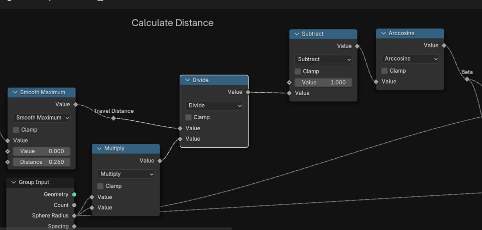
Now that we know how to increase the distance, we can plug this into our previous chunk of nodes that calculates the X, Y, Z coordinates of the point and we're good to go!

12. Final animation render setup

I thought this was a really interesting pattern to create an abstract animation with. So let's look at what it took to make this look nice.

Here's a screencast of me walking through the full setup:

This was just one example of using the Golden Ratio / Golden Angle. I think there are many more interesting ways to use the Fibonacci sequence and the Golden Ratio to create beautiful 3D art in Blender.

I hope this article has given you some inspiration to try it out and render something amazing yourself :)

Downloads

If you want to play around in the final .blend files after each stage, you can download them here:

1. Flat pattern: blendergrid-fibonacci-pattern-1-flat.blend
2. Spherical pattern: blendergrid-fibonacci-sphere-2-spherical.blend
3. Final production render: blendergrid-fibonacci-sphere-3-production-render.blend

Happy blending ☕️